
“We ought then to regard the present state of the universe as the effect of its anterior state and as the cause of the one which is to follow. Given for one instant an intelligence which could comprehend all the forces by which nature is animated and the respective situation of the beings who compose it – an intelligence sufficiently vast to submit these data to analysis – it would embrace in the same formula the motions of the greatest bodies of the universe and those of the lightest atom; for it nothing would be uncertain and the future, as the past, would be present to its eyes.”
— Pierre-Simon Laplace
The study of strategy has evolved historically from the seminal works of Machiavelli, Sun Tzu and Kautilya on the art of war, to the paradigms of game theorists like Von Neumann and Nash (Oestreicher, 2007). A philosophical thread running through these works is the characterization of strategic interactions between complex entities as chaotic. Any discussion of strategic interaction should begin with the concepts of chaos and determinism – two conflicting notions that defy consolidated explanation. In the truest sense, chaos represents disorder while determinism implies transitivity or equality. The first formal analysis of chaos is attributed to Henri Poincaré, who discovered “the phenomenon of sensitivity to initial conditions” (Smith, 1990). Poincaré’s insights on chaos posed a puzzle rather than an impasse, and the assumptions around chaos have resulted in much confusion in understanding, making it one of the deepest scientific mysteries.
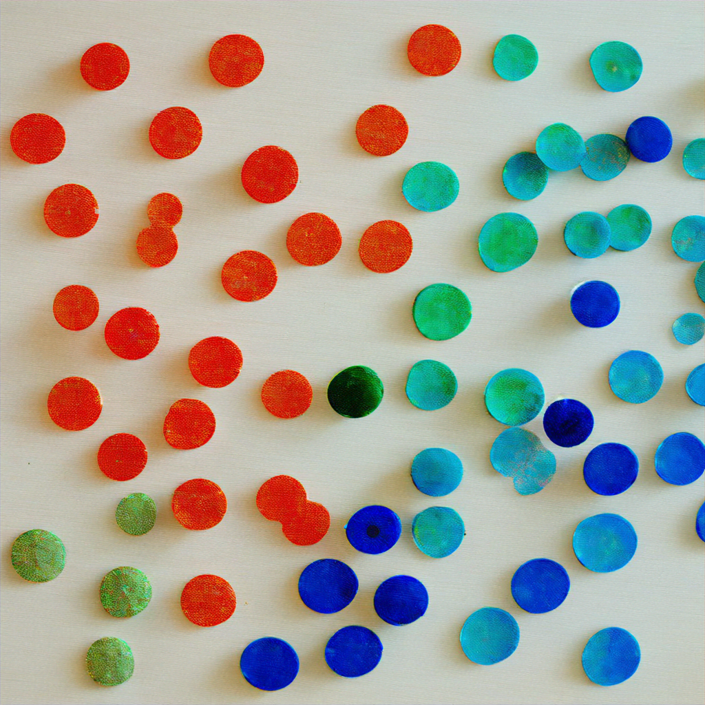
The concept of the “butterfly effect” exemplifies the intriguing properties of chaotic dynamics (Smith, 1990). A key feature is the high sensitivity to initial conditions in dynamic systems. An illustrative experiment involves a pendulum suspended over three magnets arranged in a triangle (see Figure X). Regardless of the initial release point, the pendulum eventually comes to rest hovering over one of the magnets. The initial release point is marked blue, red or green based on the final position – blue if it ends up over the blue magnet, red if over the red magnet, etc. Mapping these colored points reveals the sensitivity to initial conditions. In a discrete map of all release points (Figure Y estimates this as an illustration), the areas directly above the magnets are solid colors (blue, red and green respectively).

The uniformly colored regions are limited to the area of magnetic influence. Beyond this, the regularity in the colored dots disappears into mixed areas showing combined dependence (blue-red, blue-green, red-green) that influences the pendulum’s final position. Thus, the map also contains points sensitive to the combined influence of multiple magnets. While mixed color areas exhibit deterministic chaos in the long run, they also display experimental predictability – the effects of mixed magnetic perturbations can be predicted for each release case. However, unpredictability and sensitivity persist for regions with combined influence, as all release points experience mixed magnetic flux. This makes sensitivity to initial conditions an inherent feature of the system.
Smith (1990) describes an exceptional case of “hypersensitivity” where a steel ball rolls to the vertex of an A-shaped wedge (see Figure Z). Using equations of motion and friction properties, the ball’s potential paths can be determined – it may fall back down the right inclined plane, or forward down the left. Hypothetically, if the ball came to rest exactly at the vertex, its future path would be unpredictable. As Smith notes, the ball’s path could not be predicted regardless of reducing observational error margins. Such hypersensitive points feature even in simple systems exhibiting sensitivity to initial conditions and observational intolerance. Consider a modified ball-wedge system in an airtight box, with the vertex electromagnetized to hold the metallic ball at the tip. Gradually reducing the electromagnetic flux, at some point the ball would slip – again creating hypersensitive instability. With gravity, friction, electromagnetism and unknown atmospheric pressure, predicting the ball’s path requires modeling all forces and system properties at all spatial points and times, except the vertex tip. Replacing the wedge with a smooth cone, the ball could slip on any tangent from base to apex, amplifying hypersensitivity. Thus, certain areas of dynamic systems lack explanation against physical backdrops. While these unknowns currently defy modeling, solving them may provide new perspectives on the nature of reality.

Sensitive dependence on initial conditions is indicative of chaos (Smith, 1998). Chaos represents disorder or confusion. In their discussion of determinism in physics pertaining to “physical disorder”, Clark and Butterfield (1987) find the remarks of James Clerk Maxwell fitting: “Confusion, like the correlative term order, is not a property of material things in themselves, but only in relation to the mind which perceives them.”
Oestreicher’s (2007) historical overview of chaos theory finds mathematical closure in Socolar (2006), who introduces basic terminology of nonlinear dynamics and expands upon them to elucidate chaos. Drawing on concepts analyzed in Smith (1990), Clark and Butterfield (1987), Smith (1998), Oestreicher (2007), and Socolar (n.d.), the first hints of strategy in chaotic interactions can be brought out.
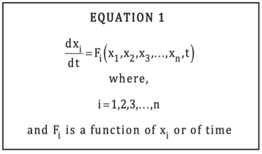
Smith (1990) proposed a mathematical modeling approach to describe phenomena through an ordered set of real variables xi. The dynamics or temporal evolution of an event or system configuration can be described by a set of smooth differential functions {Fi(xi, t)}. Given data on the xi variables of the event at a particular time point, the differential equations govern how the system’s configuration evolves over time (see Equation 1).
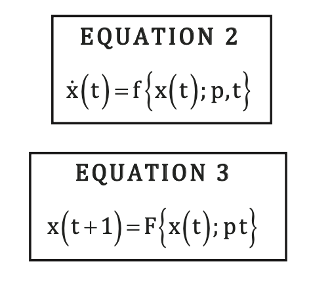
A related modeling approach using parameters was introduced by Socolar (year). Continuous time-dynamical systems can be represented as shown in Equation 2, where the vector components xi denote system variables and f is a function describing the system dynamics at fixed parameter values p. For discrete time-dynamical systems (Equation 3), the function F maps the changes in system variables over discrete time steps pt.
Equation 4 provides a geometric interpretation of the scientific modeling paradigms introduced previously, represented in an n-dimensional phase space of x with variable units over a defined time period. The resulting phase space trajectories depict the evolution of the system and can be analyzed to characterize dynamic phenomena. A spatial approximation of Equation 1 from Socolar (2006) is utilized to model spatially-extended systems, where each system variable is considered a function of space and time.
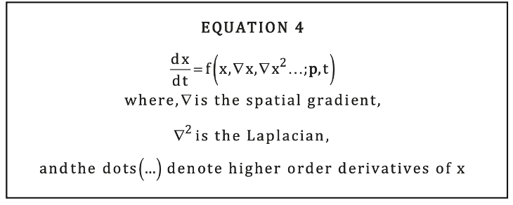
In Equation 4, the parameters p may correspond to either externally imposed position-dependent functions or environmental variables that become system variables. The former case applies when the system evolves in an inhomogeneous environment, while the latter case occurs when environmental variables are incorporated as internal system variables in a homogeneous environment (Socolar, 2006).
There are some ambiguities in the mathematical modeling frameworks described above that require examination:
- Collecting data on the variable parameters for a mathematically defined model produces time evolution trajectories of a dynamic system from precise initial conditions. Sensitivity to initial conditions is therefore an inherent aspect of mathematical modeling, where raw data inputs selected at a moment in time significantly influence the resulting behavior over time. Studying the trajectories from different initial conditions exposes points of sensitivity and hypersensitivity that introduce randomness into the system’s time evolution, seen as curves that appear to follow unpredictable chaotic paths (Smith, 1990; Socolar, 2006).
- This raises questions around the unpredictability of the analysis itself – could such turbulent dynamics be a flaw of the mathematical model, or should sensitivity to initial conditions be a default expectation of dynamic models? (Smith, 1990). Equation 1 contains a mathematical inclusion that provides an important clue about what needs to be determined. In Equations 1, 2, and 3, the functions are defined over x. However, in Equation 1 the dynamical function Fi includes an additional constraint over time. This mathematical inclusion of time in Equation 1 aligns with the following statement by Clark & Butterfield (1987): “…since a physical theory may well involve a parameter defined using a probability measure which itself evolves deterministically with time.”
- Under this assumption, the notion of sensitivity to initial conditions takes on a significantly abstract form, bordering on a concept confined purely to mathematics in general. In a deterministic framework, an observed state always has dynamic existence. If two different systems restricted to the same “dynamical laws” appear in different observed states later in time, despite identical initial observed states, it can only imply an underlying flaw or incompleteness in the mathematical model’s principles. Yet since mathematical laws defining physical systems can predict later dynamic states relatively accurately from initial parameter inputs, the only possibility is that the model does not completely encapsulate the past, present, and future observational states of the system. In a practical sense, such incompleteness is reasonable because scientific analyses occur over finite periods, notwithstanding previous or future states of the system under study (Clark & Butterfield, 1987).
- Importantly, this exemplifies the collision between deterministic and non-deterministic philosophies, the “hidden variable” aspect undermining determinism. Oestreicher (2007) draws a similar distinction, stating mathematical models’ “continuity in time and space” assumption should not apply in “cognitive neuroscience of perception” where finite time constraints exist. Thus, despite mathematical models only enabling an incomplete understanding of reality or truth of phenomena, how does one address nature’s sensitivity or hypersensitivity? Randomness is a hallmark of complexity. Absolute chaos constitutes strategic interactions between variable entities at infinite scales. Analyzing systems with many degrees of freedom poses greater challenges for nonlinearity. Large-scale interactions between defining variables become visible in spatial and network structures. Although numerous techniques can handle spatial structures, no universal principle exists to address spatiotemporal natural behavior. Certain logical techniques facilitate network analysis; for instance, Boolean functions approximate complex differential equations of biological networks like genetic regulation. Random Boolean networks or “Kauffman nets” randomize gene logical relations using binary variables representing differential equation sets. A similar complex network representation approach is Feigenbaum’s use of logistic maps to elucidate period doubling routes to chaos (Oestreicher 2007; Socolar 2006).
A broad assumption may hold that logical relations constitute strategies specific to interacting variable entities, homogeneous or heterogeneous, which conduct self-sustaining phenomena. As an example, swarm behavior exemplifies a significant self-sustaining phenomenon whereby cognitive elements seek strategic equilibrium with the environment to achieve global behavior. Thus, a guiding principle to strategic natural interactions may exist that enables cognitive elements to survive and evolve. The search for such a governing principle of strategic interactions arrives at a singular universal code underlying any strategic communication – equilibrium. The following chapter discusses equilibrium in strategic interactions by introducing the exemplary concept of Nash equilibrium.
Refer to Oestreicher (2007) and Socolar (2006) for key characteristics of linear and nonlinear systems to conceptually comprehend chaos, strange attractors, fractal time, and Lyapunov exponents. A grasp of these concepts would prove useful when comprehending the final mathematical proof presented in this work.
References
[1] Oestreicher, C. (2007). A history of chaos theory. Dialogues in Clinical Neuroscience, 9(3), 279-289.
[2] Smith, P. (1990). The Butterfly Effect. Proceedings of the Aristotelian Society. 91, pp. 247-267. Oxford University Press. Retrieved April 23, 2017, from https:// www.jstor.org/stable/4545139
[3] Clark, P, Butterfield, J. (1987). Determinism and Probability in Physics. Proceedings of the Aristotelian Society. 61, pp. 185-244. Aristotelian Society Supplementary Volume.
[4] Socolar, E.S.J. (2006). Nonlinear Dynamical Systems. In T. &. Deisboeck (Ed.), Complex Systems Science in Biomedicine (pp. 115-140). Springer.